12 List of in-built functions

The following is a complete list of the default functions which are built into Pyxplot. Except where stated otherwise, functions may be assumed to expect numerical arguments. Where arguments are represented by the letter $x$ , they must usually be real numbers. Where arguments are represented by the letter $z$ , they are usually permitted to be complex numbers. Functions which are defined within Pyxplot’s default modules, but which are not in its default namespace, are listed in subsections below.

abs( $z$ )
The abs( $z$ ) function returns the absolute magnitude of $z$ , where $z$ may be any general complex number. The output shares the physical dimensions of $z$ , if any.

acos( $z$ )
The acos( $z$ ) function returns the arccosine of $z$ , where $z$ may be any general dimensionless complex number. The output has physical dimensions of angle.

acosec( $z$ )
The acosec( $z$ ) function returns the arccosecant of $z$ , where $z$ may be any general dimensionless complex number. The output has physical dimensions of angle.

acosech( $z$ )
The acosech( $z$ ) function returns the hyperbolic arccosecant of $z$ , where $z$ may be any general dimensionless complex number. The output is dimensionless.

acosh( $z$ )
The acosh( $z$ ) function returns the hyperbolic arccosine of $z$ , where $z$ may be any general dimensionless complex number. The output is dimensionless.

acot( $z$ )
The acot( $z$ ) function returns the arccotangent of $z$ , where $z$ may be any general dimensionless complex number. The output has physical dimensions of angle.

acoth( $z$ )
The acoth( $z$ ) function returns the hyperbolic arccotangent of $z$ , where $z$ may be any general dimensionless complex number. The output is dimensionless.

acsc( $z$ )
The acsc( $z$ ) function returns the arccosecant of $z$ , where $z$ may be any general dimensionless complex number. The output has physical dimensions of angle.

acsch( $z$ )
The acsch( $z$ ) function returns the hyperbolic arccosecant of $z$ , where $z$ may be any general dimensionless complex number. The output is dimensionless.

airy_ai( $z$ )
The airy_ai( $z$ ) function returns the Airy function Ai evaluated at $z$ , where $z$ may be any dimensionless complex number.

airy_ai_diff( $z$ )
The airy_ai_diff( $z$ ) function returns the first derivative of the Airy function Ai evaluated at $z$ , where $z$ may be any dimensionless complex number.

airy_bi( $z$ )
The airy_bi( $z$ ) function returns the Airy function Bi evaluated at $z$ , where $z$ may be any dimensionless complex number.

airy_bi_diff( $z$ )
The airy_bi_diff( $z$ ) function returns the first derivative of the Airy function Bi evaluated at $z$ , where $z$ may be any dimensionless complex number.

arg( $z$ )
The arg( $z$ ) function returns the argument of the complex number $z$ , which may have any physical dimensions. The output has physical dimensions of angle.

asec( $z$ )
The asec( $z$ ) function returns the arcsecant of $z$ , where $z$ may be any general dimensionless complex number. The output has physical dimensions of angle.

asech( $z$ )
The asech( $z$ ) function returns the hyperbolic arcsecant of $z$ , where $z$ may be any general dimensionless complex number. The output is dimensionless.

asin( $z$ )
The asin( $z$ ) function returns the arcsine of $z$ , where $z$ may be any general dimensionless complex number. The output has physical dimensions of angle.

asinh( $z$ )
The asinh( $z$ ) function returns the hyperbolic arcsine of $z$ , where $z$ may be any general dimensionless complex number. The output is dimensionless.

atan( $z$ )
The atan( $z$ ) function returns the arctangent of $z$ , where $z$ may be any general dimensionless complex number. The output has physical dimensions of angle.

atan2( $x,y$ )
The atan2( $x,y$ ) function returns the arctangent of $x/y$ . Unlike atan( $y/x$ ), atan2( $x,y$ ) takes account of the signs of both $x$ and $y$ to remove the degeneracy between $(1,1)$ and $(-1,-1)$ . $x$ and $y$ must be real numbers, and must have matching physical dimensions.

atanh( $z$ )
The atanh( $z$ ) function returns the hyperbolic arctangent of $z$ , where $z$ may be any general dimensionless complex number. The output is dimensionless.

besseli( $l,x$ )
The besseli( $l,x$ ) function evaluates the $l$ th regular modified spherical Bessel function at $x$ . $l$ must be a positive dimensionless real integer. $x$ must be a real dimensionless number.

besselI( $l,x$ )
The besselI( $l,x$ ) function evaluates the $l$ th regular modified cylindrical Bessel function at $x$ . $l$ must be a positive dimensionless real integer. $x$ must be a real dimensionless number.

besselj( $l,x$ )
The besselj( $l,x$ ) function evaluates the $l$ th regular spherical Bessel function at $x$ . $l$ must be a positive dimensionless real integer. $x$ must be a real dimensionless number.

besselJ( $l,x$ )
The besselJ( $l,x$ ) function evaluates the $l$ th regular cylindrical Bessel function at $x$ . $l$ must be a positive dimensionless real integer. $x$ must be a real dimensionless number.

besselk( $l,x$ )
The besselk( $l,x$ ) function evaluates the $l$ th irregular modified spherical Bessel function at $x$ . $l$ must be a positive dimensionless real integer. $x$ must be a real dimensionless number.

besselK( $l,x$ )
The besselK( $l,x$ ) function evaluates the $l$ th irregular modified cylindrical Bessel function at $x$ . $l$ must be a positive dimensionless real integer. $x$ must be a real dimensionless number.

bessely( $l,x$ )
The bessely( $l,x$ ) function evaluates the $l$ th irregular spherical Bessel function at $x$ . $l$ must be a positive dimensionless real integer. $x$ must be a real dimensionless number.

besselY( $l,x$ )
The besselY( $l,x$ ) function evaluates the $l$ th irregular cylindrical Bessel function at $x$ . $l$ must be a positive dimensionless real integer. $x$ must be a real dimensionless number.

beta( $a,b$ )
The beta( $a,b$ ) function evaluates the beta function $B(a,b)$ , where $a$ and $b$ must be dimensionless real numbers.

call( $f,a$ )
The call( $f,a$ ) function calls the function $f$ with the arguments contained in the list $a$ .

ceil( $x$ )
The ceil( $x$ ) function returns the smallest integer value greater than or equal to $x$ , where $x$ must be a dimensionless real number.

chr( $x$ )
The chr( $x$ ) function returns the character with numerical ASCII code $x$ .

classOf( $x$ )
The classOf( $x$ ) function returns the class prototype of the object x, where $x$ may be of any object type.

cmp( $a,b$ )
The cmp( $a,b$ ) function returns $1$ if $a>b$ , $-1$ if $a<b$ and zero if $a=b$ .

cmyk( $c,m,y,k$ )
The cmyk( $c,m,y,k$ ) function returns a color object with the specified CMYK components in the range 0–1.

conjugate( $z$ )
The conjugate( $z$ ) function returns the complex conjugate of the complex number $z$ , which may have any physical dimensions.

copy( $o$ )
The copy( $o$ ) function returns a copy of the data structure $o$ , which may be of any object type. Nested data structures are not copied; see deepcopy( $o$ ) for this.

cos( $z$ )
The cos( $z$ ) function returns the cosine of $z$ , where $z$ may be any complex number and must either have physical dimensions of angle or be a dimensionless number, in which case it is understood to be measured in radians.

cosec( $z$ )
The cosec( $z$ ) function returns the cosecant of $z$ , where $z$ may be any complex number and must either have physical dimensions of angle or be a dimensionless number, in which case it is understood to be measured in radians.

cosech( $z$ )
The cosech( $z$ ) function returns the hyperbolic cosecant of $z$ , where $z$ may be any complex number and must either have physical dimensions of angle or be a dimensionless number, in which case it is understood to be measured in radians.

cosh( $z$ )
The cosh( $z$ ) function returns the hyperbolic cosine of $z$ , where $z$ may be any complex number and must either have physical dimensions of angle or be a dimensionless number, in which case it is understood to be measured in radians.

cot( $z$ )
The cot( $z$ ) function returns the cotangent of $z$ , where $z$ may be any complex number and must either have physical dimensions of angle or be a dimensionless number, in which case it is understood to be measured in radians.

coth( $z$ )
The coth( $z$ ) function returns the hyperbolic cotangent of $z$ , where $z$ may be any complex number and must either have physical dimensions of angle or be a dimensionless number, in which case it is understood to be measured in radians.

cross( $a,b$ )
The cross( $a,b$ ) function returns the vector cross product of the three-component vectors $a$ and $b$ .

csc( $z$ )
The csc( $z$ ) function returns the cosecant of $z$ , where $z$ may be any complex number and must either have physical dimensions of angle or be a dimensionless number, in which case it is understood to be measured in radians.

csch( $z$ )
The csch( $z$ ) function returns the hyperbolic cosecant of $z$ , where $z$ may be any complex number and must either have physical dimensions of angle or be a dimensionless number, in which case it is understood to be measured in radians.

deepcopy( $o$ )
The deepcopy( $o$ ) function returns a deep copy of the data structure $o$ , copying also any nested data structures. $o$ may be of any object type.

degrees( $x$ )
The degrees( $x$ ) function takes a real input which should either have physical units of angle, or be dimensionless, in which case it is assumed to be measured in radians. The output is the dimensionless number of degrees in $x$ .

diff_dx( $e,x,step$ )
The diff_dx( $e,x,step$ ) function numerically differentiates an expression $e$ with respect to $a$ at $x$ , using a step size of $step$ . ‘x’ can be replaced by any variable name of fewer than 16 characters, and so, for example, the diff_dfoobar() function differentiates an expression with respect to the variable foobar. The expression $e$ may optionally be enclosed in quotes. Both $x$ , and the output differential, may be complex numbers with any physical unit. The step size may optionally be omitted, in which case a value of $10^{-6}$ is used. The following example would differentiate the expression $x^2$ with respect to $x$ :
print diff_dx("x**2", 1, 1e-6).

ellipticintE( $k$ )
The ellipticintE( $k$ ) function evaluates the following complete elliptic integral:

$E(k) = \int _0^1 \sqrt {\frac{1-k^2 t^2}{1-t^2}}\, \mathrm{d}t.$

ellipticintK( $k$ )
The ellipticintK( $k$ ) function evaluates the following complete elliptic integral:

$K(k) = \int _0^1 \frac{\mathrm{d}t}{\sqrt {(1-t^2)(1-k^2 t^2)}}.$

ellipticintP( $k,n$ )
The ellipticintP( $k,n$ ) function evaluates the following complete elliptic integral:

$P(k,n) = \int _0^{\nicefrac {\pi }{2}} \frac{\mathrm{d}\theta }{(1+n\sin ^2\theta )(1-k^2\sin ^2\theta )}.$

erf( $x$ )
The erf( $x$ ) function evaluates the error function at $x$ , where $x$ must be a dimensionless real number.

erfc( $x$ )
The erfc( $x$ ) function evaluates the complementary error function at $x$ , where $x$ must be a dimensionless real number.

eval( $s$ )
The eval( $s$ ) function evaluates the string expression $s$ and returns the result.

exp( $z$ )
The exp( $z$ ) function returns $e^ z$ , where $z$ can be a complex number but must either be dimensionless or be an angle.

expint( $n,x$ )
The expint( $n,x$ ) function evaluates the following integral:

$\int _{t=1}^{t=\infty } \exp (-xt)/t^ n \, \mathrm{d}t.$

$n$ must be a positive real dimensionless integer and $x$ must be a real dimensionless number.

expm1( $x$ )
The expm1( $x$ ) function accurately evaluates $\exp (x)-1$ , where $x$ must be a dimensionless real number.

factors( $x$ )
The factors( $x$ ) function returns a list of the factors of the integer $x$ .

finite( $x$ )
The finite( $x$ ) function returns one if $x$ is a finite number, and zero otherwise.

floor( $x$ )
The floor( $x$ ) function returns the largest integer value smaller than or equal to $x$ , where $x$ must be a dimensionless real number.

gamma( $x$ )
The gamma( $x$ ) function evaluates the gamma function $\Gamma (x)$ , where $x$ must be a dimensionless real number.

gcd(...)
The gcd(...) function returns the greatest common divisor (a.k.a. highest common factor) of its arguments, which should be dimensionless non-zero positive integers.

globals()
The globals() function returns a dictionary of all currently-defined global variables.

gray( $x$ )
The gray( $x$ ) function returns color object representing a shade of gray with brightness $x$ in the range 0–1.

grey( $x$ )
The grey( $x$ ) function returns color object representing a shade of gray with brightness $x$ in the range 0–1.

hcf(...)
The hcf(...) function returns the highest common factor (a.k.a. greatest common divisor) of its arguments, which should be dimensionless non-zero positive integers.

heaviside( $x$ )
The heaviside( $x$ ) function returns the Heaviside function, defined to be one for $x\geq 0$ and zero otherwise. $x$ must be a dimensionless real number.

hsb( $h,s,b$ )
The hsb( $h,s,b$ ) function returns color object with specified hue, saturation and brightness in the range 0–1.

hyperg_0F1( $c,x$ )
The hyperg_0F1( $c,x$ ) function evaluates the hypergeometric function $_0F_1(c,x)$ . All inputs must be dimensionless real numbers. For reference, the implementation used is GSL’s gsl_sf_hyperg_0F1 function.

hyperg_1F1( $a,b,x$ )
The hyperg_1F1( $a,b,x$ ) function evaluates the hypergeometric function $_1F_1(a,b,x)$ . All inputs must be dimensionless real numbers. For reference, the implementation used is GSL’s gsl_sf_hyperg_1F1 function.

hyperg_2F0( $a,b,x$ )
The hyperg_2F0( $a,b,x$ ) function evaluates the hypergeometric function $_2F_0(a,b,x)$ . All inputs must be dimensionless real numbers.For reference, the implementation used is GSL’s gsl_sf_hyperg_2F0 function.

hyperg_2F1( $a,b,c,x$ )
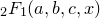The hyperg_2F1( $a,b,c,x$ ) function evaluates the hypergeometric function $_2F_1(a,b,c,x)$ . All inputs must be dimensionless real numbers. For reference, the implementation used is GSL’s gsl_sf_hyperg_2F1 function. This implementation cannot evaluate the region $|x|<1$ .

hyperg_U( $a,b,x$ )
The hyperg_U( $a,b,x$ ) function evaluates the hypergeometric function $U(a,b,x)$ . All inputs must be dimensionless real numbers. For reference, the implementation used is GSL’s gsl_sf_hyperg_U function.

hypot(...)
The hypot(...) function returns the quadrature sum of its arguments, $\sqrt {x^2+y^2+\ldots }$ . Its arguments must be numerical, but may have any physical dimensions so long as they match. They can be complex numbers.

Im( $z$ )
The Im( $z$ ) function returns the imaginary part of the complex number $z$ , which may have any physical units. The number returned shares the same physical units as $z$ .

int_dx( $e,min,max$ )
The int_dx( $e,min,max$ ) function numerically integrates an expression $e$ with respect to $x$ between $min$ and $max$ . ‘x’ can be replaced by any variable name of fewer than 16 characters, and so, for example, the int_dfoobar() function integrates an expression with respect to the variable foobar. The expression $e$ may optionally be enclosed in quotes. $min$ and $max$ may have any physical units, so long as they match, but must be real numbers. The output integral may be a complex number, and may have any physical dimensions. The following example would integrate the expression $x^2$ with respect to $x$ between $1$ m and $2$ m:
print int_dx("x**2", 1*unit(m), 2*unit(m)).

jacobi_cn( $u,m$ )
The jacobi_cn( $u,m$ ) function evaluates a Jacobi elliptic function; it returns the value $\cos \phi$ where $\phi$ is defined by the integral

$\int _{0}^{\phi }\frac{\mathrm{d}\theta }{\sqrt {1-m\sin ^2\theta }}.$

jacobi_dn( $u,m$ )
The jacobi_dn( $u,m$ ) function evaluates a Jacobi elliptic function; it returns the value $\sqrt {1-m\sin ^2\theta }$ where $\phi$ is defined by the integral

$\int _{0}^{\phi }\frac{\mathrm{d}\theta }{\sqrt {1-m\sin ^2\theta }}.$

jacobi_sn( $u,m$ )
The jacobi_sn( $u,m$ ) function evaluates a Jacobi elliptic function; it returns the value $\sin \phi$ where $\phi$ is defined by the integral

$\int _{0}^{\phi }\frac{\mathrm{d}\theta }{\sqrt {1-m\sin ^2\theta }}.$

lambert_W0( $x$ )
The lambert_W0( $x$ ) function evaluates the principal real branch of the Lambert W function, for which $W>-1$ when $x<0$ .

lambert_W1( $x$ )
The lambert_W1( $x$ ) function evaluates the secondary real branch of the Lambert W function, for which $W<-1$ when $x<0$ .

lcm(...)
The lcm(...) function returns the lowest common multiple of its arguments, which should be dimensionless positive integers.

ldexp( $x,y$ )
The ldexp( $x,y$ ) function returns $x$ times $2^ y$ for integer y, where both $x$ and $y$ must be real.

legendreP( $l,x$ )
The legendreP( $l,x$ ) function evaluates the $l$ th Legendre polynomial at $x$ , where $l$ must be a positive dimensionless real integer and $x$ must be a real dimensionless number.

legendreQ( $l,x$ )
The legendreQ( $l,x$ ) function evaluates the $l$ th Legendre function at $x$ , where $l$ must be a positive dimensionless real integer and $x$ must be a real dimensionless number.

len( $o$ )
The len( $o$ ) function returns the length of the object $o$ . The may be the length of a string, or the number of entries in a compound data type.

ln( $z$ )
The ln( $z$ ) function returns the natural logarithm of $z$ , where $z$ may be any complex dimensionless number.

locals()
The locals() function returns a dictionary of all currently-defined local variables in the present scope.

log( $z$ )
The log( $z$ ) function returns the natural logarithm of $z$ , where $z$ may be any complex dimensionless number.

log10( $z$ )
The log10( $z$ ) function returns the logarithm to base 10 of $z$ , where $z$ may be any complex dimensionless number.

logn( $x,n$ )
The logn( $x,n$ ) function returns the logarithm of $x$ to base $n$ .

lrange([ $f$ ], $l$ ,[ $s$ ])
The lrange([ $f$ ], $l$ ,[ $s$ ]) function returns a vector of numbers between $f$ and $l$ with uniform multiplicative spacing $s$ . If not specified, $f=1$ and $s=2$ . If two arguments are specified, these are interpreted as $f$ and $l$ . The arguments $f$ and $l$ may have any physical units, so long as they match. $s$ must be a dimensionless number.

matrix(...)
The matrix(...) function creates a new matrix object. See types.matrix.

max(...)
The max(...) function returns the highest-valued of its arguments, which may be of any object type and may have any physical dimensions, so long as they match. If either input is complex, the input with the larger magnitude is returned. If a single vector or list object is supplied, the highest-valued item in the vector or list is returned.

min(...)
The min(...) function returns the lowest-valued of its arguments, where may be of any object type and may have any physical dimensions, so long as they match. If either input is complex, the input with the smaller magnitude is returned. If a single vector or list object is supplied, the lowest-valued item in the vector or list is returned.

mod( $x,y$ )
The mod( $x,y$ ) function returns the remainder of $x/y$ , where $x$ and $y$ may have any physical dimensions so long as they match but must both be real.

module(...)
The module(...) function creates a new module object. See types.module.

open( $x$ [, $y$ ])
The open( $x$ [, $y$ ]) function opens the file $x$ with string access mode $y$ , and returns a file handle object.

ord( $s$ )
The ord( $s$ ) function returns the ASCII code of the first character of the string $s$ .

ordinal( $x$ )
The ordinal( $x$ ) function returns an ordinal string, for example, “1st”, “2nd” or “3rd”, for any positive dimensionless real number $x$ .

pow( $x,y$ )
The pow( $x,y$ ) function returns $x$ to the power of $y$ , where $x$ and $y$ may both be complex numbers and $x$ may have any physical dimensions but $y$ must be dimensionless. It not not permitted for $y$ to be complex if $x$ is not dimensionless, since this would lead to an output with complex physical dimensions.

prime( $x$ )
The prime( $x$ ) function returns one if floor( $x$ ) is a prime number and zero otherwise.

primeFactors( $x$ )
The primeFactors( $x$ ) function returns a list of the prime factors of the integer $x$ .

radians( $x$ )
The radians( $x$ ) function takes a real input which should either have physical units of angle, or be dimensionless, in which case it is assumed to be measured in degrees. The output is the dimensionless number of radians in $x$ .

raise( $e,s$ )
The raise( $e,s$ ) function raises the exception $e$ , with error string $s$ . $e$ should be an exception object; $s$ should be an error message string.

range([ $f$ ], $l$ ,[ $s$ ])
The range([ $f$ ], $l$ ,[ $s$ ]) function returns a vector of uniformly-spaced numbers between $f$ and $l$ , with stepsize $s$ . If not specified, $f=0$ and $s=1$ . If two arguments are specified, these are interpreted as $f$ and $l$ . The arguments may have any physical units, so long as they match.

Re( $z$ )
The Re( $z$ ) function returns the real part of the complex number $z$ , which may have any physical units. The number returned shares the same physical units as $z$ .

rgb( $r,g,b$ )
The rgb( $r,g,b$ ) function returns a color object with specified RGB components in the range 0–1.

romanNumeral( $x$ )
The romanNumeral( $x$ ) function returns the Roman numeral representing the number $x$ , for any positive dimensionless real input less than 10,000.

root( $z,n$ )
The root( $z,n$ ) function returns the $n$ th root of $z$ . $z$ may be any complex number, and may have any physical dimensions. $n$ must be a dimensionless integer. When complex arithmetic is enabled, and whenever $z$ is positive, this function is entirely equivalent to pow(z,1/n). However, when $z$ is negative and complex arithmetic is disabled, the expression pow(z,1/n) may not be evaluated, since it will in general have a small imaginary part for any finite-precision floating-point representation of $1/n$ . The expression root(z,n), on the other hand, may be evaluated under such conditions, providing that $n$ is an odd integer.

round( $x$ )
The round( $x$ ) function rounds the value $x$ to the nearest integer. If $x$ is exactly halfway between integers, it is rounded away from zero. $x$ must be a dimensionless real number.

sec( $z$ )
The sec( $z$ ) function returns the secant of $z$ , where $z$ may be any complex number and must either have physical dimensions of angle or be a dimensionless number, in which case it is understood to be measured in radians.

sech( $z$ )
The sech( $z$ ) function returns the hyperbolic secant of $z$ , where $z$ may be any complex number and must either have physical dimensions of angle or be a dimensionless number, in which case it is understood to be measured in radians.

sgn( $x$ )
The sgn( $x$ ) function returns 1 if x is greater than zero, -1 if x is less than zero, and 0 if x equals zero.

sin( $z$ )
The sin( $z$ ) function returns the sine of $z$ , where $z$ may be any complex number and must either have physical dimensions of angle or be a dimensionless number, in which case it is understood to be measured in radians.

sinc( $z$ )
The sinc( $z$ ) function returns the sinc function $\sin (z)/z$ for any complex number $z$ , which may either be dimensionless, in which case it is understood to be measured in radians, or have physical dimensions of angle. The result is dimensionless.

sinh( $z$ )
The sinh( $z$ ) function returns the hyperbolic sine of $z$ , where $z$ may be any complex number and must either have physical dimensions of angle or be a dimensionless number, in which case it is understood to be measured in radians.

sqrt( $z$ )
The sqrt( $z$ ) function returns the square root of $z$ , which may be any complex number and may have any physical dimensions.

sum(...)
The sum(...) function returns the sum of its arguments, which be of any object type, and may have any physical units, so long as it is possible to add them together.

tan( $z$ )
The tan( $z$ ) function returns the tangent of $z$ , where $z$ may be any complex number and must either have physical dimensions of angle or be a dimensionless number, in which case it is understood to be measured in radians.

tanh( $z$ )
The tanh( $z$ ) function returns the hyperbolic tangent of $z$ , where $z$ may be any complex number and must either have physical dimensions of angle or be a dimensionless number, in which case it is understood to be measured in radians.

texify( $s$ )
The texify( $s$ ) function takes a string representation of an algebraic expression as its input, e.g. “(x/3)**2”, and returns a latex representation of it.

texifyText( $s$ )
The texifyText( $s$ ) function returns a string of latex text corresponding to the supplied text string, with any reserved characters escaped.

tophat( $x,\sigma$ )
The tophat( $x,\sigma$ ) function returns one if $|x| \leq |\sigma |$ , and zero otherwise. Both inputs must be real, but may have any physical dimensions so long as they match.

typeOf( $o$ )
The typeOf( $o$ ) function returns the type of the object $o$ .

unit(…)
The unit(…) function multiplies a number by a physical unit. The string inside the brackets should consist of a string of the names of physical units, multiplied together with the * operator, divided using the / operator, or raised by numeric powers using the operator. The list may be commenced with a numeric constant, for example: unit(2*m2/s).

vector(...)
The vector(...) function creates a new vector object. See types.vector.

zernike( $n,m,r,\phi$ )
The zernike( $n,m,r,\phi$ ) function evaluates the Zernike polynomial $Z^ m_ n(r,\phi )$ , where $m$ and $n$ are non-negative integers with $n\geq m$ , $r$ is the radial coordinate in the range $0<r<1$ and $\phi$ is the azimuthal coordinate.

zernikeR( $n,m,r$ )
The zernikeR( $n,m,r$ ) function evaluates the radial Zernike polynomial $R^ m_ n(r)$ , where $m$ and $n$ are non-negative integers with $n\geq m$ and $r$ is the radial coordinate in the range $0<r<1$ .

zeta( $x$ )
The zeta( $x$ ) function evaluates the Riemann zeta function for any dimensionless number $x$ .