7.8 Subroutines
Subroutines are similar to mathematical functions (see Section 4.3), and once defined, can be used anywhere in algebraic expressions, just as functions can be. However, instead of being defined by a single algebraic expression, whenever a subroutine is evaluated, a block of Pyxplot commands of arbitrary length is executed. This gives much greater flexibility for implementing complex algorithms. Subroutines are defined using the following syntax:
subroutine <name>(<variable1>,...)
 {
  ...
  return <value>
 }
Where name is the name of the subroutine, variable1 is an argument taken by the subroutine, and the value passed to the return statement is the value returned to the caller. Once the return statement is reached, execution of the subroutine is terminated. The following two examples would produce entirely equivalent results:
f(x,y) = x*sin(y)

subroutine f(x,y)
 {
  return x*sin(y)
 }
In either case, the function/subroutine could be evaluated by typing:
print f(1,pi/2)
If a subroutine ends without any value being returned using the return statement, then a value of zero is returned.
Subroutines may serve one of two purposes. In many cases they are used to implement complicated mathematical functions for which no simple algebraic expression may be given. Secondly, they may be used to repetitively execute a set of commands whenever they are required. In the latter case, the subroutine may not have a return value, but may merely be used as a mechanism for encapsulating a block of commands. In this case, the call command may be used to execute a subroutine, discarding any return value which it may produce, as in the example:
pyxplot> subroutine f(x,y) { print "%s - %s = %s"%(x,y,x-y) ; }
pyxplot> call f(2,1)
2 - 1 = 1
pyxplot> call f(5*unit(inch), 10*unit(mm))
127 mm - 10 mm = 117 mm
Newton fractals are formed by iterating the equation
![\[ z_{n+1} = z_ n - \frac{f(z_ n)}{f^\prime (z_ n)}, \]](images/img-0304.png) |
 , where
  is any complex number and
  is any mathematical function. This series is the Newton-Raphson method for numerically finding solutions to the equation
  , and with time usually converges towards one such solution for well-behaved functions. The complex number represents the initial guess at the position of the solution being sought. The Newton fractal is formed by asking which solution the iteration converges upon, as a function of the position of the initial guess in the complex plane. In the case of the cubic polynomial
  , which has three solutions, a map might be generated with points colored red, green or blue to represent convergence towards the three roots.
 If
is close to one of the roots, then convergence towards that particular root is guaranteed, but further afield the map develops a fractal structure. In this example, we define a Pyxplot subroutine to produce such a map as a function of  , and then plot the resulting map using the colormap plot style (see Section 8.12). To make the fractal prettier – it contains, after all, only three colors as strictly defined – we vary the brightness of each point depending on how many iterations are required before the series ventures within a distance of
  of any of the roots
  .
. set numerics complex
set unit angle nodimensionless
root1 = exp(i*unit( 0*deg))
root2 = exp(i*unit(120*deg))
root3 = exp(i*unit(240*deg))
tolerance = 1e-2
subroutine newtonFractal(x,y)
{
global iter
z = x+i*y
iter = 0
while (1)
{
z = z - (z**3-1)/(3*z**2)
if abs(z-root1)
 tolerance { ; return 1 ; }
if abs(z-root2)
tolerance { ; return 2 ; }if abs(z-root3)
tolerance { ; return 3 ; }iter = iter + 1
}
}
# Plot Newton fractal
set size square
set key below
set xrange [-1.5:1.5]
set yrange [-1.5:1.5]
set sample grid 250x250
set colmap hsb(c1*0.667,0.8+0.2*c2,1.0-0.8*c2)
set nocolkey
set log c2
plot newtonFractal(x,y):iter+2 with colormap
![\includegraphics[width=8cm]{examples/eps/ex_newton}](images/img-0313.png)
The equation of motion for a pendulum bob may be derived from the rotational analogue to Newton’s Second Law,
 where
where  is torque,
  is moment of inertia and
  is the displacement of the pendulum bob from the vertical. For a pendulum of length
  , with a bob of mass
  , this equation becomes
  . In the small-angle approximation, such that
  , it reduces to the equation for simple harmonic motion, with the solution
 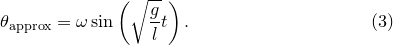 |
(7.1) |
A more exact solution requires integration of the second-order differential equation of motion including the
 term. This integral cannot be done analytically, but the solution can be written in the form
 ![\begin{equation} \theta _\mathrm {exact}(t) = 2\sin ^{-1}\left[ k\, \mathrm{sn}\left(\sqrt {\frac{g}{l}}t,k\right)\right]. \label{eq:pendulum_ exact} \end{equation}](images/img-0323.png) |
(7.2) |
where
 is a Jacobi elliptic function and
  . The Jacobi elliptic function cannot be analytically computed, but can be numerically approximated using the jacobi_sn(u,m) function in Pyxplot.
 Below, we produce a plot of Equations () and (). The horizontal axis is demarcated in units of the dimensionless period of the pendulum to eliminate
 and , and a swing amplitude of
  is assumed:
 set unit angle nodimensionless
theta_approx(a,t) = a*sin(2*pi*t)
theta_exact (a,t) = 2*asin(sin(a/2)*jacobi_sn(2*pi*t,sin(a/2)))
set unit of angle degrees
set key below
set xlabel r’Time / $
 sqrt{g/l}$’
set ylabel r’$
theta$’omega = unit(30*deg)
plot [0:4] theta_approx(omega,x) title ’Approximate solution’,
theta_exact (omega,x) title ’Exact solution’
![\includegraphics[width=9cm]{examples/eps/ex_pendulum}](images/img-0329.png)
As is apparent, at this amplitude, the exact solution begins to deviate noticeably from the small-angle solution within 2–3 swings of the pendulum. We now seek to quantify more precisely how long the two solutions take to diverge by defining a subroutine to compute how long
 it takes before the two solutions to deviate by some amount
  . We then plot these times as a function of amplitude
  for three deviation thresholds. Because this subroutine takes a significant amount of time to run, we only compute 40 samples for each value of :
 subroutine pendulumDivergenceTime(omega, deviation)
{
for t=0 to 20 step 0.05
{
approx = theta_approx(omega,t)
exact = theta_exact (omega,t)
if (abs(approx-exact)
 deviation) { ;break; }
}
return t
}
set key top right
set xlabel r’Amplitude of swing’
set ylabel r’Time / $
sqrt{g/l}$ taken to diverge’set samples 40
plot [unit(5*deg):unit(30*deg)][0:19]
pendulumDivergenceTime(x,unit(20*deg)) title r"$20
 circ$ deviation",
 pendulumDivergenceTime(x,unit(10*deg)) title r"$10
circ$ deviation", pendulumDivergenceTime(x,unit( 5*deg)) title r"$ 5
circ$ deviation" ![\includegraphics[width=9cm]{examples/eps/ex_pendulum2}](images/img-0334.png)