5.10 Random data generation

Pyxplot has functions for generating random numbers from a variety of common probability distributions. These functions are in the random module:

random.random() – returns a random real number between 0 and 1.
random.binomial() – returns a random sample from a binomial distribution with $n$ independent trials and a success probability $p$ .
random.chisq() – returns a random sample from a $\chi$ -squared distribution with $\nu$ degrees of freedom.
random.gaussian() – returns a random sample from a Gaussian (normal) distribution of standard deviation $\sigma$ and centred on zero.
random.lognormal() – returns a random sample from the log normal distribution centred on $\zeta$ , and of width $\sigma$ .
random.poisson() – returns a random integer from a Poisson distribution with mean $n$ .
random.tdist() – returns a random sample from a $t$ -distribution with $\nu$ degrees of freedom.

These functions all rely on a common underlying random number generator¹, whose seed may be set using the set seed command, which should be followed by any integer. The sequence of random samples generated is always the same after setting any particular seed.

When Pyxplot starts, the seed is implicitly set to zero. This means that Pyxplot always produces the same series of random numbers when restarted. This series can be reproduced by typing:

set seed 0

For applications where this repeatability is undesirable, the following command may help, using the system clock as a random seed:

set seed time.now().toUnix()

This gives a different sequence of random numbers each second. However, the user is advised to consider carefully whether this is sufficient for the particular application being implemented.

Example: Using random numbers to estimate the value of $\pi$

Pyxplot’s functions for generating random numbers are most commonly used for adding noise to artificially-generated data. In this example, however, we use them to implement a rather inefficient algorithm for estimating the value of the mathematical constant $\pi$ . The algorithm works by spreading randomly-placed samples in the square $\left\{ -1<x<1;\; -1<y<1\right\}$ . The number of these which lie within the circle of unit radius about the origin are then counted. Since the square has an area of $4\, \mathrm{unit}^2$ and the circle an area of $\pi \, \mathrm{unit}^2$ , the fraction of the points which lie within the unit circle equals the ratio of these two areas: $\pi /4$ .
The following script performs this calculation using $N=5000$ randomly placed samples. Firstly, the positions of the random samples are generated using the random() function, and written to a file called random.dat using the tabulate command. Then, the foreach datum command – which will be introduced in Section 7.4 – is used to loop over these, counting how many lie within the unit circle.
Nsamples = 500

rand() = random.random()

set samp Nsamples
set output "pi_estimation.dat"
tabulate 1-2*rand():1-2*rand() using 0:2:3

n=0
foreach datum i,j in "pi_estimation.dat" u 2:3
{
  n = n + (hypot(i,j)1)
}
print "pi=%s"%(n / Nsamples * 4)
On the author’s machine, this script returns a value of $3.1352$ when executed using the random samples which are returned immediately after starting Pyxplot. This method of estimating $\pi$ is well modelled as a Poisson process, and the uncertainty in this result can be estimated from the Poisson distribution to be $1/\sqrt {N}$ . In this case, the uncertainty is $0.01$ , in close agreement with the deviation of the returned value of $3.1352$ from more accurate measures of $\pi$ .
With a little modification, this script can be adapted to produce a diagram of the datapoints used in its calculation. Below is a modified version of the second half of the script, which loops over the data points stored in the data file random.dat. It uses Pyxplot’s vector graphics commands, which will be introduced in Chapter 10, to produce such a diagram:
set multiplot ; set nodisplay

# Draw a unit circle and a unit square
title = "ex_pi_estimation" ; load "fig_init.ppl"
box from -width/2,-width/2 to width/2,width/2
circle at 0,0 radius width/2 with lt 2

# Now plot the positions of these random data points andi
# count how many lie within a unit circle
n=0
foreach datum i,j in "pi_estimation.dat" using 2:3
{
  point at width/2*i , width/2*j with ps 0.1
  n = n + (hypot(i,j)1)
}
set display ; refresh
print "pi=%.4f"%(n / Nsamples * 4)
The graphical output from this script is shown below. The number of datapoints has been reduced to Nsamples $=500$ for clarity:
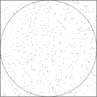
$\includegraphics{examples/eps/ex_pi_estimation}$

Footnotes

The gsl library’s default random number generator, gsl_rng_default is used. As of version 1.15, this maps to gsl_rng_mt19937 with a default seed of zero. The various probability distributions above are sampled using the functions gsl_ran_binomial and similar.