Pyxplot Users' Guide: Linked axes

8.8.9 Linked axes

Often it may be desired that multiple axes on a graph share a common range, or be related to one another by some algebraic expression. For example, a plot with wavelength $\lambda$ of light as one axis may usefully also have parallel axes showing frequency of light $\nu =c/\lambda$ or photon energy $E=hc/\lambda$ . The following example sets the x2 axis to share a common range with the x axis:

set axis x2 linked x

An algebraic relationship between two axes may be set by stating the algebraic relationship after the keyword using, as in the following example which implement the formulae shown above for the frequency and energy of photons of light as a function of their wavelength:

set xrange [200*unit(nm):unit(800*nm)]
set axis x2 linked x1 using phy.c/x
set axis x3 linked x2 using phy.h*x

As in the set xformat command, a dummy variable of x, y or z is used in the linkage expression depending on the direction of the axis being linked to, but a dummy variable of x is still used when linking to, for example, the x2 axis.

As these examples demonstrate, the functions used to link axes need not be linear. In fact, axes with any arbitrary mapping between position and value can be produced by linked in a non-linear fashion to another linear axis, which, if desired, can then be hidden using the set axis invisible command. Multi-valued mappings are also permitted. Any data plotted against the following x2-axis for a suitable range of x-axis

set axis x2 linked x1 using x**2

would appear twice, symmetrically on either side of $x=0$ .

Insofar as is possible, linked axes autoscale intelligently when no range is set. Thus, if the x2-axis is linked to the x-axis, and no range to set for the x-axis, the x-axis will autoscale to include all of the data plotted against both itself and the x2-axis. Similarly, if the x2-axis is linked to the x-axis by means of some algebraic expression, the x-axis will attempt to autoscale to include the data plotted against the x2-axis, though in some cases – especially with non-monotonic linking functions – this may prove too difficult. Where Pyxplot detects that it has failed, a warning is issued recommending that a hard range be set for – in this example – the x-axis.

Example: A plot of many blackbodies demonstrating the use of linked axes

In this example we produce a plot of blackbody spectra for five different temperatures $T$ , using the Planck formula

$B_\nu (\nu ,T)=\left(\frac{2h^3}{c^2}\right)\frac{\nu ^3}{\exp (h\nu /kT)-1}$

which is evaluated in Pyxplot by the system-defined mathematical function Bv(nu,T). We use the axis linkage commands listed as an example in the text of Section 8.8.9 to produce three parallel horizontal axes showing wavelength of light, frequency of light and photon energy.
set numeric display latex
set unit angle nodimensionless
set log x y
set key bottom right
set ylabel  "Flux density" ; set unit preferred W/Hz/m**2/sterad
set x1label "Wavelength"
set x2label "Frequency"     ; set unit of frequency Hz
set x3label "Photon Energy" ; set unit of energy eV
set axis x2 linked x1 using phy.c/x
set axis x3 linked x2 using phy.h*x
set xtics unit(0.1*um),10
set x2tics 1e12*unit(Hz),10
set x3tics 0.01*unit(eV),10
set xrange [80*unit(nm):unit(mm)]
set yrange [1e-20*unit(W/Hz/m**2/sterad):]

bb(wlen,T) = phy.Bv(phy.c/wlen,T)

plot bb(x,  30) title r"$T=  30$,K",
     bb(x, 100) title r"$T= 100$,K",
     bb(x, 300) title r"$T= 300$,K",
     bb(x,1000) title r"$T=1000$,K",
     bb(x,3000) title r"$T=3000$,K"
$\includegraphics[width=10cm]{examples/eps/ex_multiaxes}$

Example: A plot of the temperature of the CMBR as a function of redshift demonstrating non-linear axis linkage

In this example we produce a plot of the temperature of the cosmic microwave background radiation (CMBR) as a function of time $t$ since the Big Bang, on the x-axis, and equivalently as a function of redshift $z$ , on the x2-axis. The specialist cosmology function ast_Lcdm_z(,,,) is used to make the highly non-linear conversion between time $t$ and redshift $z$ , adopting some standard values for the cosmological parameters $H_0$ , $\Omega _\mathrm {M}$ and $\Omega _\Uplambda$ . Because the temperature of the CMBR is most easily expressed as a function of redshift as 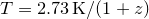$T=2.73\, \mathrm{K}/(1+z)$ , we plot this function against axis x2.
h0 = 70
omega_m = 0.27
omega_l = 0.73
age = ast.Lcdm_age(h0,omega_m,omega_l)
set xrange [0.01*age:0.99*age]
set xtics (unit(1*Gyr),unit(4*Gyr),unit(7*Gyr),unit(10*Gyr),unit(13.6*Gyr))
set unit of time Gyr
set axis x2 linked x using ast.Lcdm_z(age-x,h0,omega_m,omega_l)
set xlabel "Time since Big Bang $t$"
set ylabel "CMBR Temperature $T$"
set x2label "Redshift $z$"
plot unit(2.73*K)*(1+x) ax x2y1
$\includegraphics[width=8cm]{examples/eps/ex_cmbrtemp}$