8.6 Plotting parametric functions

Parametric functions are functions expressed in forms such as

	$\displaystyle x$	$\displaystyle =$	$\displaystyle r \sin (t)$
	$\displaystyle y$	$\displaystyle =$	$\displaystyle r \cos (t) ,$

where separate expressions are supplied for the ordinate and abscissa values as a function of some free parameter $t$ . The above example is a parametric representation of a circle of radius $r$ . Before Pyxplot can usefully plot parametric functions, it is generally necessary to stipulate the range of values of $t$ over which the function should be sampled. This may be done using the set trange command, as in the example

set trange [unit(0*rad):unit(2*pi*rad)]

or in the plot command itself. By default, values in the range $0\leq t\leq 1$ are used. Note that the set trange command differs from other commands for setting axis ranges in that auto-scaling is not an allowed behaviour; an explicit range must be specified for $t$ .

Having set an appropriate range for $t$ , parametric functions may be plotted by placing the keyword parametric before the list of functions to be plotted, as in the following simple example which plots a circle:

set trange [unit(0*rev):unit(1*rev)]
plot parametric sin(t):cos(t)

Optionally, a range for $t$ can be specified on a plot-by-plot basis immediately after the keyword parametric, and thus the effect above could also be achieved using:

plot parametric [unit(0*rev):unit(1*rev)] sin(t):cos(t)

The only difference between parametric function plotting and ordinary function plotting – other than the change of dummy variable from x to t – is that one fewer column of data is generated. Thus, whilst

plot f(x)

generates two columns of data, with values of $x$ in the first column,

plot parametric f(t)

generates only one column of data.

Example: Spirograph patterns

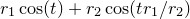
Spirograph patterns are produced when a pen is tethered to the end of a rod which rotates at some angular speed $\omega _1$ about the end of another rod, which is itself rotating at some angular speed $\omega _2$ about a fixed central point. Spirographs are commonly implemented mechanically as wheels within wheels – epicycles within deferents, mathematically speaking – but in this example we implement them using the parametric functions

	$\displaystyle x$	$\displaystyle =$	$\displaystyle r_1 \sin (t) + r_2 \sin (t r_1 / r_2)$
	$\displaystyle y$	$\displaystyle =$	$\displaystyle r_1 \cos (t) + r_2 \cos (t r_1 / r_2)$

which are simply the sum of two circular motions with angular velocities inversely proportional to their radii. The complexity of the resulting spirograph pattern depends on how rapidly the rods return to their starting configuration; if the two chosen angular speeds for the rods have a large lowest common multiple, then a highly complicated pattern will result. In the example below, we pick a ratio of $8:15$ :
set nogrid
set nokey

r1 = 1.5
r2 = 0.8
set size square
set trange[0:40*pi]
set samples 2500
plot parametric r1*sin(t) + r2*sin(t*(r1/r2)) :
r1*cos(t) + r2*cos(t*(r1/r2))
$\includegraphics[width=8cm]{examples/eps/ex_spirograph}$
Other ratios of r1:r2 such as $7:19$ and $5:19$ also produce intricate patterns.