8.6.1 Two-dimensional parametric surfaces
Pyxplot can also plot datasets which can be parameterised in terms of two free parameters  and
and  . This is most often useful in conjunction with the surface plot style, allowing any
  -surface to be plotted (see Section 8.14.1 for details of the surface plot style). However, it also works in conjunction with any other plot style, allowing, for example, -grids of points to be constructed.
As in the case of parametric lines above, the range of values that each free parameter should take must be specified. This can be done using the set urange and set vrange commands. These commands also act to switch Pyxplot between one- and two-dimensional parametric function evaluation; whilst the set trange command indicates that the next parametric function should be evaluated along a single raster of values of  , the set urange and set vrange commands indicate that a grid of values should be used. By default, the range of values used for and is
  .
.
The number of samples to be taken can be specified using a command of the form
set sample grid 20x50
which specifies that 20 different values of and 50 different values of should be used, yielding a total of 1000 datapoints. The following example uses the lines plot style to generate a sequence of cross-sections through a two-dimensional Gaussian surface:
set num err quiet
set nokey
set size 7 square
set sample grid 20x20
set urange [-1:1] ; set vrange [-1:1]
set xrange [-1.1:1.1]
f(u,v) = 0.4*exp(-(u**2+v**2)/0.2)
plot parametric u:v+f(u,v) with l
![\includegraphics[width=8cm]{examples/eps/ex_datagrid}](images/img-0443.png)
The ranges of values to use for and may alternatively be specified on a dataset-by-dataset basis within the plot command, as in the example
plot parametric [0:1][0:1] u:v , \
     parametric [0:1] sin(t):cos(t)
In this example we plot a torus, which can be parametrised in terms of two free parameters
and as  |
 |
 |
|||
 |
|
 |
|||
 |
|
 |
and both run in the range ![$[0:2\pi ]$](images/img-0449.png) ,
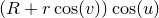
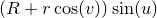
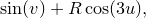
,  is the distance of the tube’s center from the center of the torus, and
  is the radius of the tube.
 R = 3
r = 0.5
f(u,v) = (R+r*cos(v))*cos(u)
g(u,v) = (R+r*cos(v))*sin(u)
h(u,v) = r*sin(v)
set urange [0:2*pi]
set vrange [0:2*pi]
set zrange [-2.5:2.5]
set nokey
set size 8 square
set grid
set sample grid 50x20
plot 3d parametric f(u,v):g(u,v):h(u,v) with surf fillcol blue
![\includegraphics[width=8cm]{examples/eps/ex_torus}](images/img-0452.png)
In this example we plot a trefoil knot, which is the simplest non-trivial knot in topology. Simply put, this means that it is not possible to untie the knot without cutting it. The knot follows the line
|
|
 |
|||
|
|
 |
|||
|
|
 |
|
|
 |
|||
|
|
 |
|||
|
|
 |
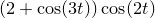
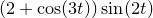
and run in the ranges and ![$[-\pi :\pi ]$](images/img-0460.png) respectively, and and determine the size and thickness of the knot as in an analogous fashion to the previous example.
respectively, and and determine the size and thickness of the knot as in an analogous fashion to the previous example. r = 5
R = 2
f(u,v) = cos(2*u)*cos(v) + r*cos(2*u)*(1.5+sin(3*u)/2)
g(u,v) = sin(2*u)*cos(v) + r*sin(2*u)*(1.5+sin(3*u)/2)
h(u,v) = sin(v)+R*cos(3*u)
set urange [0:2*pi]
set vrange [-pi:pi]
set nokey
set size 8 square
set grid
set sample grid 150x20
plot 3d parametric f(u,v):g(u,v):h(u,v) with surf fillcol blue
![\includegraphics[width=8cm]{examples/eps/ex_trefoil}](images/img-0462.png)