Pyxplot

Download this example: script.ppl output.eps output.png

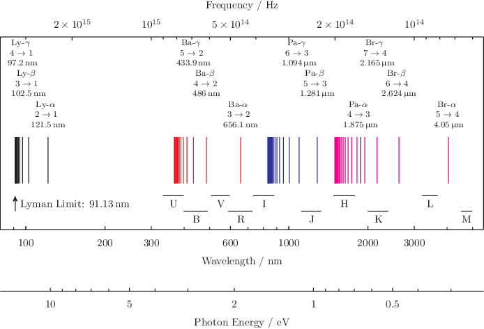
Using Pyxplot's 'set arrow' and 'set label' commands (II)

In this example, we use Pyxplot's loop constructs to produce a labelled diagram of the lines of hydrogen.

Script

set numeric display latex
set width 16
set fontsize 1
set size ratio 0.4
set numerics sf 4
set log x
set x1label "Wavelength"
set x2label "Frequency"     ; set unit of frequency Hz
set x3label "Photon Energy" ; set unit of energy eV
set axis x2 linked x1 using phy.c/x
set axis x3 linked x2 using phy.h*x
set noytics ; set nomytics

# Draw lines of first four series of hydrogen lines
an=2
n=1
foreach seriesName in ["Ly","Ba","Pa","Br"]
 {
  for m=n+1 to n+21
   {
    wl = 1/(phy.Ry*(1/n**2-1/m**2))
    set arrow an from wl,0.3 to wl,0.6 with nohead col n
    if (m-n==1) { ; greekLetter = r"\alpha" ; }
    if (m-n==2) { ; greekLetter = r"\beta"  ; }
    if (m-n==3) { ; greekLetter = r"\gamma" ; }
    if (m-n<4)
     {
      set label an r"\parbox{5cm}{\footnotesize\center{\
        %s-$%s$\newline $%d\to%d$\newline %s\newline}}" \
        %(seriesName,greekLetter,m,n,wl) at wl,0.55+0.2*(m-n) \
        hal center val center
     }
    an = an+1
   }
  n=n+1
 }

# Label astronomical photometric colors
foreach datum i,name,wl_c,wl_w in "--" using \
    1:"%s"%($2):($3*unit(nm)):($4*unit(nm))
 {
  arry = 0.12+0.1*(i%2) # Vertical positions for arrows
  laby = 0.07+0.1*(i%2) # Vertical positions for labels
  x0 = (wl_c-wl_w/2) # Shortward end of passband
  x1 =  wl_c         # Centre of passband
  x2 = (wl_c+wl_w/2) # Longward end of passband
  set arrow an from x0,arry to x2,arry with nohead
  set label an name at x1,laby hal center val center
  an = an+1
 }
 1 U  365   66
 2 B  445   94
 3 V  551   88
 4 R  658  138
 5 I  806  149
 6 J 1220  213
 7 H 1630  307
 8 K 2190  390
 9 L 3450  472
10 M 4750  460
END

# Draw a marker for the Lyman limit
ll = 91.1267*unit(nm)
set arrow 1 from ll,0.12 to ll,0.22
set label 1 "Lyman Limit: %s"%(ll) at 95*unit(nm),0.17 \
     hal left val center

# Finally produce plot
plot [80*unit(nm):5500*unit(nm)][0:1.25]