Pyxplot

Download this example: script.ppl output.eps output.png

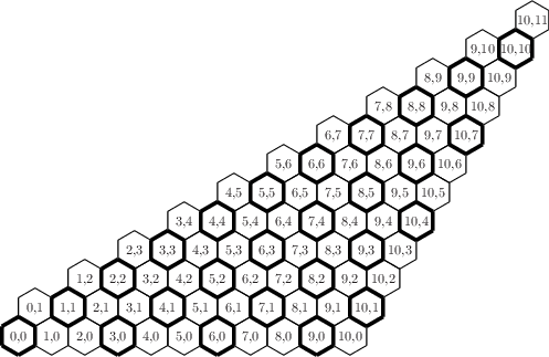
Example plot - the conductivity of nanotubes

In this example we produce a diagram of the irreducible wedge of possible carbon nanotube configurations, highlighting those configurations which are electrically conductive. We use Pyxplot's loop constructs to automate the production of the hexagonal grid which forms the basis of the diagram.

Script

basisAngleX =   0*unit(deg)
basisAngleY = 120*unit(deg)
lineLen     =   4*unit(mm)

set fontsize 0.8

# Set up a transformation matrix
transformMat = matrix([[sin(basisAngleX),sin(basisAngleY)], \
                       [cos(basisAngleX),cos(basisAngleY)] ])
transformMat *= lineLen

subroutine line(p1,p2,lw)
 {
  line from transformMat*p1 to transformMat*p2 with linewid lw
 }

subroutine hexagon(p,lw)
 {
  call line(p+vector([ 0, 0]),p+vector([ 0,-1]),lw)
  call line(p+vector([ 0,-1]),p+vector([ 1,-1]),lw)
  call line(p+vector([ 1,-1]),p+vector([ 2, 0]),lw)
  call line(p+vector([ 2, 0]),p+vector([ 2, 1]),lw)
  call line(p+vector([ 2, 1]),p+vector([ 1, 1]),lw)
  call line(p+vector([ 1, 1]),p+vector([ 0, 0]),lw)
 }

set multiplot ; set nodisplay

for x=0 to 10
 {
  for y=0 to x+1
   {
    p = vector([x+2*y , 2*x+y])
    call hexagon(p, ((x-y)%3==0)?4:1)
    text '%d,%d'%(x,y) at transformMat*(p+vector([1,0])) \
      hal cen val cen
   }
 }

set display ; refresh