Pyxplot Users' Guide: Surface plotting

8.14.1 Surface plotting

The surface plot style is similar to the colormap and contourmap plot styles, but produces maps of the values $z(x,y)$ of functions of two variables using three-dimensional surfaces. The surface is displayed as a grid of four-sided elements, whose number may be specified using the set samples command, as in the example

set samples grid 40x40

If data is supplied from a data file, then it is first re-sampled onto a regular grid using one of the methods described in Section 8.12.

The example below plots a surface indicating the magnitude of the imaginary part of $\log (x+iy)$ :

set numerics complex
set xlabel r"Re($z$)"
set ylabel r"Im($z$)"
set zlabel r"$mathrm{Im}(mathrm{log}[z])$"
set key below
set size 8 square
set grid
set view -30,30
plot 3d [-10:10][-10:10] Im(log(x+i*y))
with surface col black fillcol blue

$\includegraphics[width=10cm]{examples/eps/ex_surface_log}$

Example: A surface plotted above a contour map

In this example, we plot a surface showing the value of the expression $x^3/20+y^2$ , and project below it a series of contours in the $(x,y)$ plane.
set nokey
set size 8 square
plot 3d x**3/20+y**2 with surface col black fillc red,
x**3/20+y**2 with contours col black
$\includegraphics[width=10cm]{examples/eps/ex_surface_polynomial}$

Example: The sinc( $x$ ) function represented as a surface

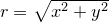In this example, we produce a surface showing the function $\mathrm{sinc}(r)$ where $r=\sqrt {x^2+y^2}$ . To produce a prettier result, we vary the color of the surface such that the hue of the surface varies with azimuthal position, its saturation varies with radius $r$ , and its brightness varies with height $z$ .
set numerics complex
set xlabel "$x$"
set ylabel "$y$"
set zlabel "$z$"
set xformat r"%s$pi$"%(x/pi)
set yformat r"%s$pi$"%(y/pi)
set xtics 3*pi ; set mxtics pi
set ytics 3*pi ; set mytics pi
set ztics
set key below
set size 8 square
set grid
plot 3d [-6*pi:6*pi][-6*pi:6*pi][-0.3:1] sinc(hypot(x,y))
with surface col black
fillcol hsb(atan2($1,$2)/(2*pi)+0.5,hypot($1,$2)/30+0.2,$3*0.5+0.5)
$\includegraphics[width=10cm]{examples/eps/ex_surface_sinc}$