C.3 Estimating the error in $\mathbf{u}^0$

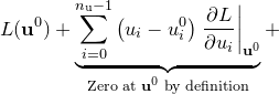
To estimate the error in the best-fitting parameter values that we find, we assume $\mathrm{P}\left( \mathbf{u} | \left\{ \mathbf{x}_ i, f_ i, \sigma _ i \right\} \right)$ to be approximated by an $n_\mathrm {u}$ -dimensional Gaussian distribution around $\mathbf{u}^0$ . Taking a Taylor expansion of $L(\mathbf{u})$ about $\mathbf{u}^0$ , we can write:

	$\displaystyle L(\mathbf{u})$	$\displaystyle =$	$\displaystyle L(\mathbf{u}^0) + \underbrace{ \sum _{i=0}^{n_\mathrm {u}-1} \left( u_ i - u^0_ i \right) \left.\frac{\partial L}{\partial u_ i}\right\|_{\mathbf{u}^0} }_{\textrm{Zero at $\mathbf{u}^0$ by definition}} + \label{eqa:L_ taylor_ expand}$		(C.4)
	$\displaystyle$	$\displaystyle$	$\displaystyle \sum _{i=0}^{n_\mathrm {u}-1} \sum _{j=0}^{n_\mathrm {u}-1} \frac{\left( u_ i - u^0_ i \right) \left( u_ j - u^0_ j \right)}{2} \left.\frac{\partial ^2 L}{\partial u_ i \partial u_ j}\right\|_{\mathbf{u}^0} + \mathcal{O}\left( \mathbf{u} - \mathbf{u}^0\right)^3 \nonumber$

Since the logarithm of a Gaussian distribution is a parabola, the quadratic terms in the above expansion encode the Gaussian component of the probability distribution $\mathrm{P}\left( \mathbf{u} | \left\{ \mathbf{x}_ i, f_ i, \sigma _ i \right\} \right)$ about $\mathbf{u}^0$ .¹ We may write the sum of these terms, which we denote $Q$ , in matrix form:

$\begin{equation} Q = \frac{1}{2} \left(\mathbf{u} - \mathbf{u}^0\right)^\mathbf {T} \mathbf{A} \left(\mathbf{u} - \mathbf{u}^0\right) \label{eqn:Q_ vector} \end{equation}$

(C.5)

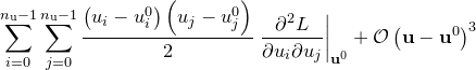
where the superscript $^\mathbf {T}$ represents the transpose of the vector displacement from $\mathbf{u}^0$ , and $\mathbf{A}$ is the Hessian matrix of $L$ , given by:

$\begin{equation} A_{ij} = \nabla \nabla L = \left.\frac{\partial ^2 L}{\partial u_ i \partial u_ j}\right|_{\mathbf{u}^0} \end{equation}$

(C.6)

This is the Hessian matrix which is output by the fit command. In general, an $n_\mathrm {u}$ -dimensional Gaussian distribution such as that given by Equation () yields elliptical contours of equi-probability in parameter space, whose principal axes need not be aligned with our chosen coordinate axes – the variables $u_0 ... u_{n_ u-1}$ . The eigenvectors $\mathbf{e}_ i$ of $\mathbf{A}$ are the principal axes of these ellipses, and the corresponding eigenvalues $\lambda _ i$ equal $1/\sigma _ i^2$ , where $\sigma _ i$ is the standard deviation of the probability density function along the direction of these axes.

This can be visualised by imagining that we diagonalise $\mathbf{A}$ , and expand Equation () in our diagonal basis. The resulting expression for $L$ is a sum of square terms; the cross terms vanish in this basis by definition. The equations of the equi-probability contours become the equations of ellipses:

$\begin{equation} Q = \frac{1}{2} \sum _{i=0}^{n_\mathrm {u}-1} A_{ii} \left(u_ i - u^0_ i\right)^2 = k \end{equation}$

(C.7)

where $k$ is some constant. By comparison with the equation for the logarithm of a Gaussian distribution, we can associate $A_{ii}$ with $-1/\sigma _ i^2$ in our eigenvector basis.

The problem of evaluating the standard deviations of our variables $u_ i$ is more complicated, however, as we are attempting to evaluate the width of these elliptical equi-probability contours in directions which are, in general, not aligned with their principal axes. To achieve this, we first convert our Hessian matrix into a covariance matrix.

Footnotes

The use of this is called Gauss’ Method. Higher order terms in the expansion represent any non-Gaussianity in the probability distribution, which we neglect. See MacKay, D.J.C., Information Theory, Inference and Learning Algorithms, CUP (2003).