C.6 Finding $\sigma _ i$

Throughout the preceding sections, the uncertainties in the supplied target values $f_ i$ have been denoted $\sigma _ i$ (see Section C.1). The user has the option of supplying these in the source datafile, in which case the provisions of the previous sections are now complete; both best-estimate parameter values and their uncertainties can be calculated. The user may also, however, leave the uncertainties in $f_ i$ unstated, in which case, as described in Section C.1, we assume all of the data values to have a common uncertainty $\sigma _\mathrm {data}$ , which is an unknown.

In this case, where $\sigma _ i = \sigma _\mathrm {data} \, \forall \, i$ , the best fitting parameter values are independent of $\sigma _\mathrm {data}$ , but the same is not true of the uncertainties in these values, as the terms of the Hessian matrix do depend upon $\sigma _\mathrm {data}$ . We must therefore undertake a further calculation to find the most probable value of $\sigma _\mathrm {data}$ , given the data. This is achieved by maximising $\mathrm{P}\left( \sigma _\mathrm {data} | \left\{ \mathbf{x}_ i, f_ i \right\} \right)$ . Returning once again to Bayes’ Theorem, we can write:

$\begin{equation} \mathrm{P}\left( \sigma _\mathrm {data} | \left\{ \mathbf{x}_ i, f_ i \right\} \right) = \frac{ \mathrm{P}\left( \left\{ f_ i \right\} | \sigma _\mathrm {data}, \left\{ \mathbf{x}_ i \right\} \right) \mathrm{P}\left( \sigma _\mathrm {data} | \left\{ \mathbf{x}_ i \right\} \right) }{ \mathrm{P}\left( \left\{ f_ i \right\} | \left\{ \mathbf{x}_ i \right\} \right) } \end{equation}$

(C.17)

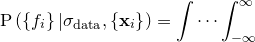
As before, we neglect the denominator, which has no effect upon the maximisation problem, and assume a uniform prior $\mathrm{P}\left( \sigma _\mathrm {data} | \left\{ \mathbf{x}_ i \right\} \right)$ . This reduces the problem to the maximisation of $\mathrm{P}\left( \left\{ f_ i \right\} | \sigma _\mathrm {data}, \left\{ \mathbf{x}_ i \right\} \right)$ , which we may write as a marginalised probability distribution over $\mathbf{u}$ :

	$\displaystyle \label{eqa:p_ f_ given_ sigma} \mathrm{P}\left( \left\{ f_ i \right\} \| \sigma _\mathrm {data}, \left\{ \mathbf{x}_ i \right\} \right) = \idotsint _{-\infty }^{\infty }$	$\displaystyle \mathrm{P}\left( \left\{ f_ i \right\} \| \sigma _\mathrm {data}, \left\{ \mathbf{x}_ i \right\} , \mathbf{u} \right) \times$	$\displaystyle$		(C.18)
	$\displaystyle$	$\displaystyle \mathrm{P}\left( \mathbf{u} \| \sigma _\mathrm {data}, \left\{ \mathbf{x}_ i \right\} \right) \, \mathrm{d}^{n_\mathrm {u}}\mathbf{u}$	$\displaystyle \nonumber$

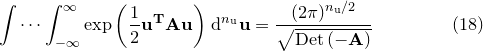
Assuming a uniform prior for $\mathbf{u}$ , we may neglect the latter term in the integral, but even with this assumption, the integral is not generally tractable, as $\mathrm{P}\left( \left\{ f_ i \right\} | \sigma _\mathrm {data}, \left\{ \mathbf{x}_ i \right\} , \left\{ \mathbf{u}_ i \right\} \right)$ may well be multimodal in form. However, if we neglect such possibilities, and assume this probability distribution to be approximate a Gaussian globally, we can make use of the standard result for an $n_\mathrm {u}$ -dimensional Gaussian integral:

$\begin{equation} \idotsint _{-\infty }^{\infty } \exp \left( \frac{1}{2}\mathbf{u}^\mathbf {T} \mathbf{A} \mathbf{u} \right) \, \mathrm{d}^{n_\mathrm {u}}\mathbf{u} = \frac{ (2\pi )^{n_\mathrm {u}/2} }{ \sqrt {\mathrm{Det}\left(-\mathbf{A}\right)} } \end{equation}$

(C.19)

We may thus approximate Equation () as:

	$\displaystyle \mathrm{P}\left( \left\{ f_ i \right\} \| \sigma _\mathrm {data}, \left\{ \mathbf{x}_ i \right\} \right)$	$\displaystyle \approx$	$\displaystyle \mathrm{P}\left( \left\{ f_ i \right\} \| \sigma _\mathrm {data}, \left\{ \mathbf{x}_ i \right\} , \mathbf{u}^0 \right) \times$		(C.20)
	$\displaystyle$	$\displaystyle$	$\displaystyle \mathrm{P}\left( \mathbf{u}^0 \| \sigma _\mathrm {data}, \left\{ \mathbf{x}_ i, f_ i \right\} \right) \frac{ (2\pi )^{n_\mathrm {u}/2} }{ \sqrt {\mathrm{Det}\left(-\mathbf{A}\right)} } \nonumber$

As in Section C.2, it is numerically easier to maximise this quantity via its logarithm, which we denote $L_2$ , and can write as:

	$\displaystyle L_2$	$\displaystyle =$	$\displaystyle \sum _{i=0}^{n_\mathrm {d}-1} \left( \frac{ -\left[f_ i - f_{\mathbf{u}^0}(\mathbf{x}_ i)\right]^2 }{ 2\sigma _\mathrm {data}^2 } - \log _ e \left(2\pi \sqrt {\sigma _\mathrm {data}} \right) \right) +$		(C.21)
	$\displaystyle$	$\displaystyle$	$\displaystyle \nonumber \log _ e \left( \frac{ (2\pi )^{n_\mathrm {u}/2} }{ \sqrt {\mathrm{Det}\left(-\mathbf{A}\right)} } \right)$

This quantity is maximised numerically, a process simplified by the fact that $\mathbf{u}^0$ is independent of $\sigma _\mathrm {data}$ .